California Housing Regression with Five Models and Geographic Error Analysis
Abstract
Five regressors (Linear, Ridge, Lasso, Random Forest, Gradient Boosting) on the California Housing dataset, evaluated under 5-fold cross-validation. Tree ensembles dominate linear models by a large margin (R² 0.82 vs 0.60), revealing strong non-linear structure in the feature-to-target mapping. Permutation importance corroborates impurity-based importance and identifies median income, geographic location, and house age as the dominant predictors. A geographic error map shows where the best model still struggles: the Bay Area and the LA basin, where the dataset's 500k cap censors the upper tail of the target distribution.
Dataset
20,640 California census-tract observations, eight features:
| Feature | Meaning |
|---|---|
| MedInc | median income, tens of thousands USD |
| HouseAge | median house age in years |
| AveRooms | average rooms per household |
| AveBedrms | average bedrooms per household |
| Population | block population |
| AveOccup | average occupants per household |
| Latitude / Longitude | block centroid |
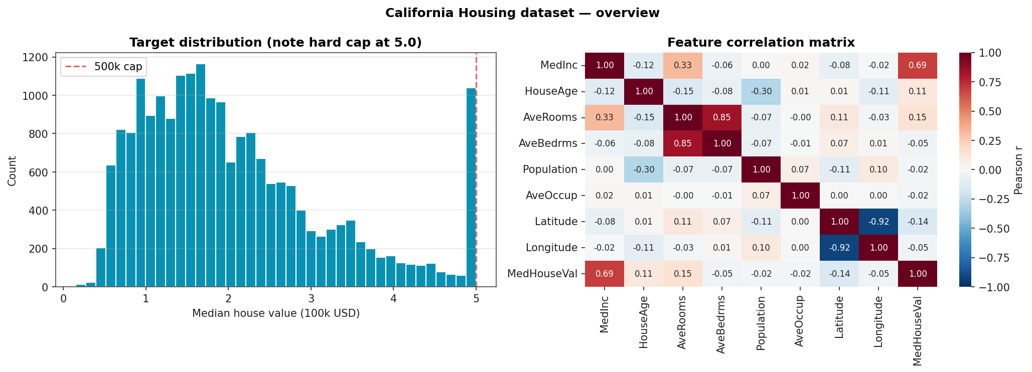
Target is the median house value of the block, scaled to units of 100k USD, capped at 5.0 (500k). The cap is visible as a spike at the right of the target histogram.
Headline Results
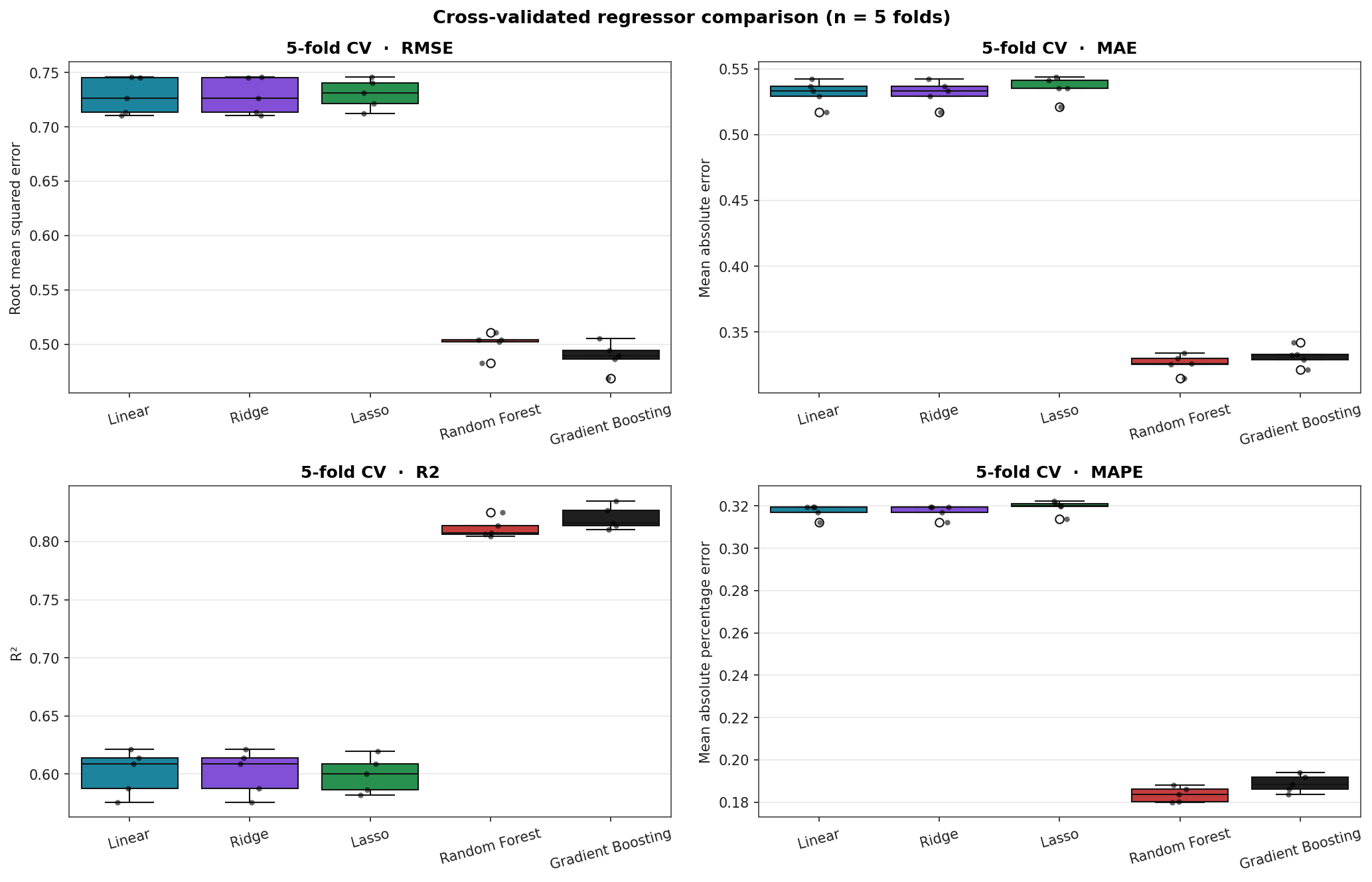
Stratified 5-fold cross-validation. RMSE and MAE in units of 100k USD; MAPE as a percentage; R² unitless.
| Model | CV RMSE | CV MAE | CV R² | CV MAPE |
|---|---|---|---|---|
| Gradient Boosting | 0.489 ± 0.013 | 0.332 | 0.820 | 18.9 % |
| Random Forest | 0.501 ± 0.011 | 0.326 | 0.811 | 18.4 % |
| Linear | 0.728 ± 0.017 | 0.532 | 0.601 | 31.8 % |
| Ridge | 0.728 ± 0.017 | 0.532 | 0.601 | 31.8 % |
| Lasso | 0.730 ± 0.014 | 0.535 | 0.599 | 31.9 % |
Tree ensembles cut RMSE by a third and MAPE roughly in half against the linear baseline. Ridge and Lasso are indistinguishable from plain Linear on this dataset because the features are not particularly collinear and there is no benefit to L1 / L2 regularisation when the linear hypothesis class is itself the bottleneck.
CV Score Distributions
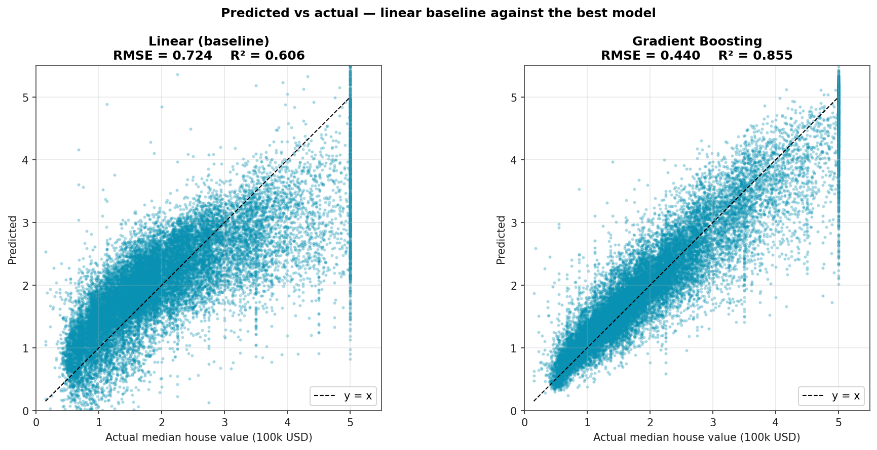
Predicted vs Actual
Linear regression vs Gradient Boosting on the same data. The linear model's predictions cluster around the mean with a clear underprediction at the upper tail; the boosted model resolves the relationship much better but still bumps up against the 500k cap (the ceiling at y = 5.0).
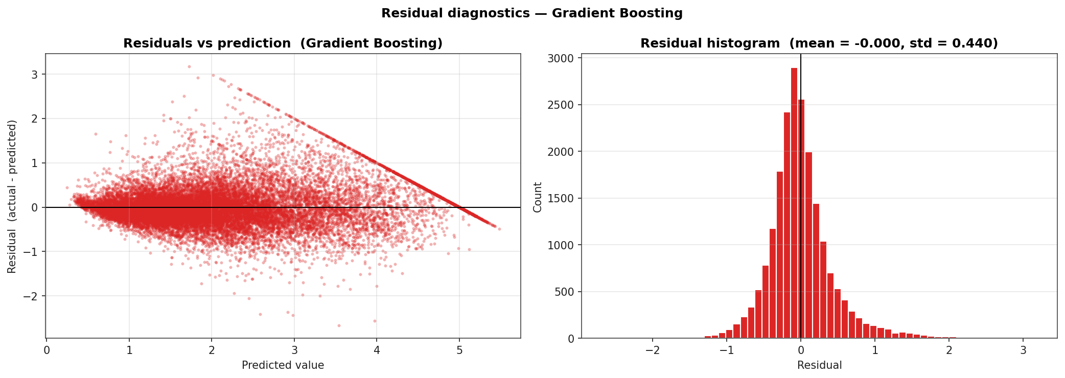
Residual Diagnostics
Residuals (actual minus predicted) for Gradient Boosting. Two structural features stand out: the residual cluster at the right of the predicted-axis is the 500k-cap effect (the model can never predict above the censoring boundary, so high-value blocks always show negative residuals); the residual histogram has a slightly heavier right tail than left, indicating modest under-prediction on the high end.
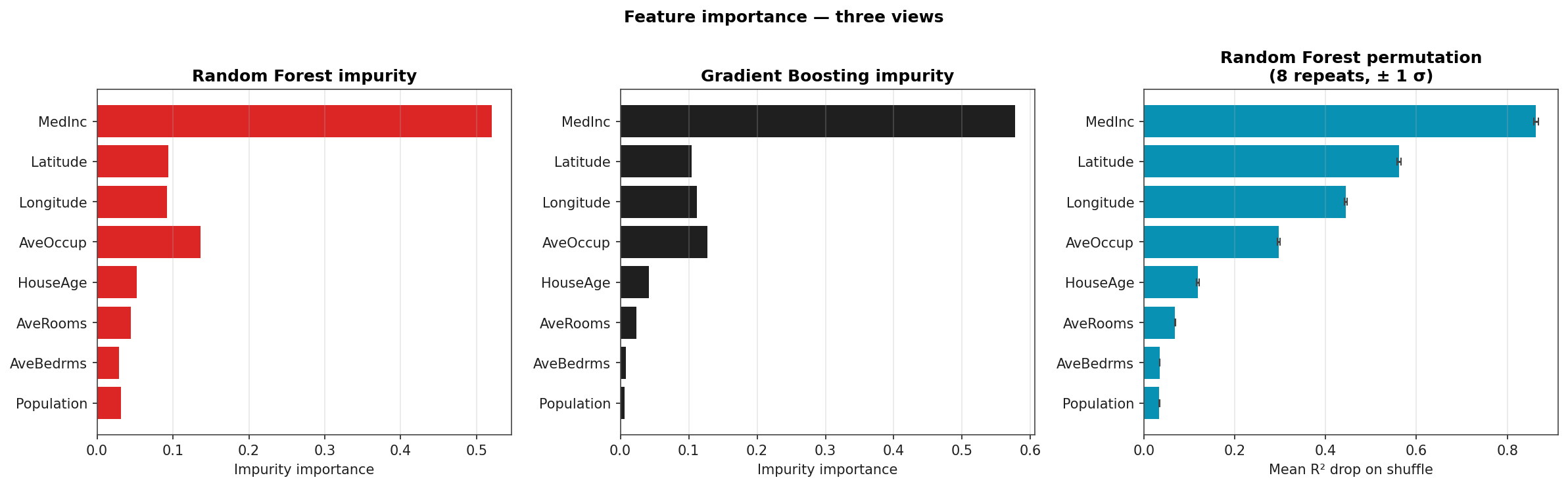
Feature Importance: Three Views
Random Forest impurity (left), Gradient Boosting impurity (middle), Random Forest permutation importance (right, eight repeats). All three orderings agree on the top three: median income, latitude, longitude. Permutation importance shrinks the role of low-cardinality features (HouseAge) relative to impurity, the well-known impurity-importance bias-correction story.
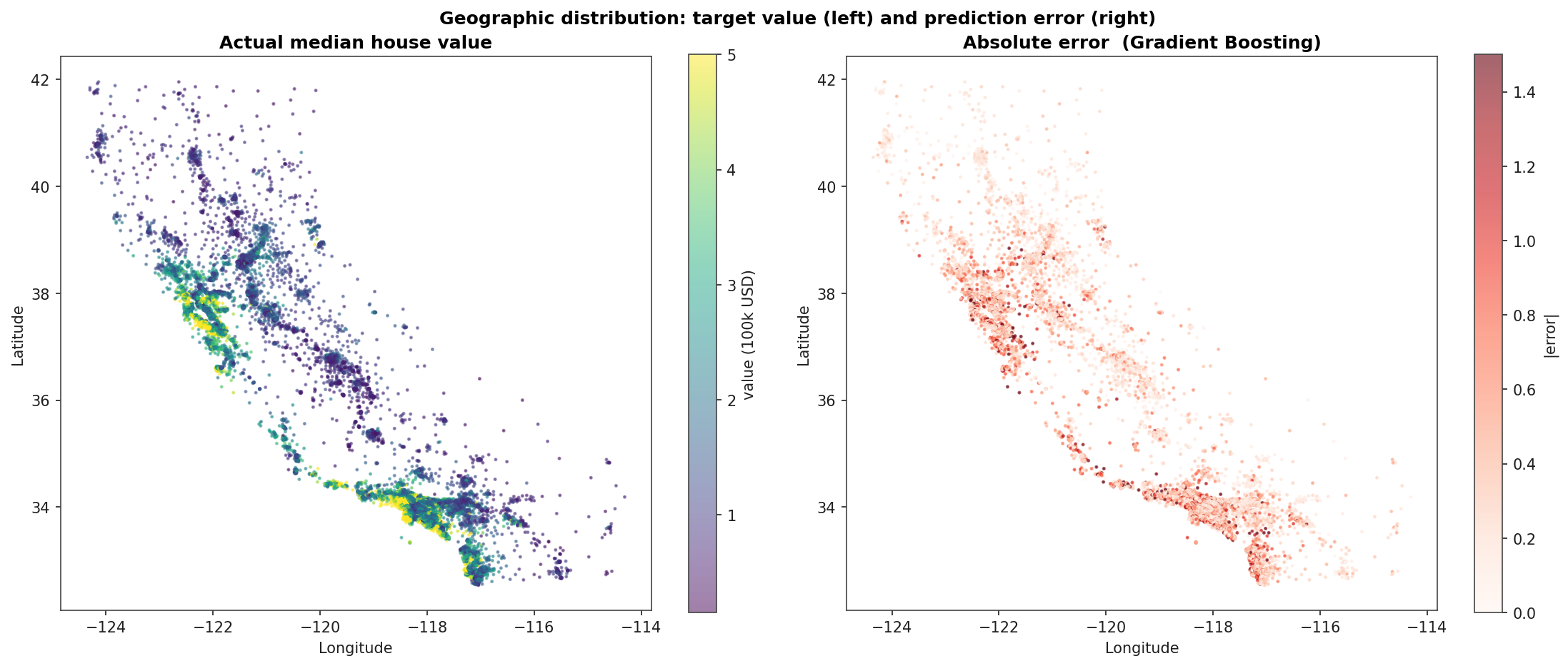
Geographic Error Map
Left: actual median house value by census block, plotted on California's coastline shape. Right: absolute error of the Gradient Boosting model on the same blocks. The error concentrates in the Bay Area and along the LA / Orange County coast: the regions where median house values frequently exceed the dataset's 500k cap and the model has no signal to fit beyond it.