Model Predictive Control · Receding-Horizon Collision Avoidance

Predictive · L-BFGS-B · Horizon Ablation

Abstract

Model predictive control replaces the gradient-flow myopia of reactive schemes with a finite-horizon optimisation: at every control step, optimise a control sequence over the next H steps that minimises a quadratic goal-tracking cost plus an exponential collision penalty, apply the first action, and re-plan. The horizon H is the knob that buys foresight at the cost of compute. This page demonstrates a 2-D point-mass MPC on the same scenario the reactive controller solves, plus an ablation showing how horizon length trades planning time for path quality and success.

Algorithm

State x = (p, v) ∈ R⁴, control u ∈ R² (acceleration). Discretise with dt = 0.1 s:

p_{k+1}  =  p_k  +  v_k · dt  +  ½ · u_k · dt²
v_{k+1}  =  v_k  +  u_k · dt
‖u_k‖    ≤  u_max

At every control step, solve

min_{u_0..u_{H-1}}   Σ_{k=1..H}  [ ‖p_k − p_goal‖²  +  λ_u · ‖u_{k-1}‖²  +  λ_obs · ϕ(p_k) ]

where  ϕ(p)  =  Σ over obstacles  max(0, ε − d_i(p))²    (collision penalty)
       d_i(p)  =  ‖p − p_obs_i‖  −  r_obs_i
       λ_u     =  0.05      (control-effort weight)
       λ_obs   =  50        (collision-penalty weight)
       ε       =  0.15 m    (safety margin)

Solver: scipy.optimize.minimize with L-BFGS-B, max 30 iterations per control step. Apply only u_0, advance the state, re-plan from the new position. The penalty term is quadratic-in-violation rather than infinite-barrier, which keeps the cost differentiable and tractable for L-BFGS.

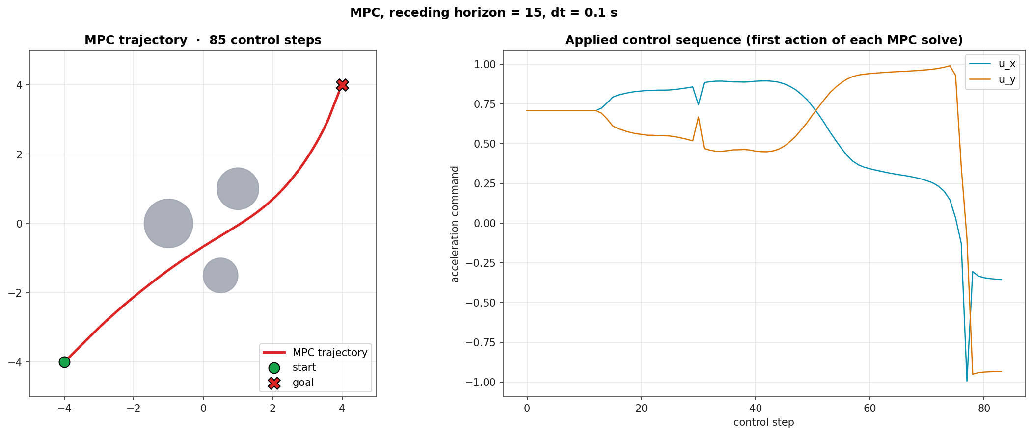
Diagnostic: Trajectory and Control

Left: MPC trajectory (red) on the same three-obstacle scenario the reactive controller solved with a smoother deflection profile. Right: applied u_x and u_y commands across the 85-step rollout, showing the controller's coordinated braking and lateral corrections.

Two-panel figure: MPC trajectory through three obstacles on the left, and the applied acceleration commands u_x and u_y over time on the right

Horizon Ablation

Same scenario, four horizons. The shortest horizon (H=3) fails: not enough lookahead to commit to a deflection, the agent oscillates around the obstacle and runs out of step budget. From H=6 onward the controller succeeds, with path length monotonically decreasing as the horizon grows. Compute scales roughly linearly in H (each MPC solve is one L-BFGS run) plus an additional factor from the larger optimisation variable count.

H	Outcome	Path length	Total compute
3	stuck	14.73	469 ms
6	success	11.67	1936 ms
10	success	11.43	7170 ms
15	success	11.31	17795 ms

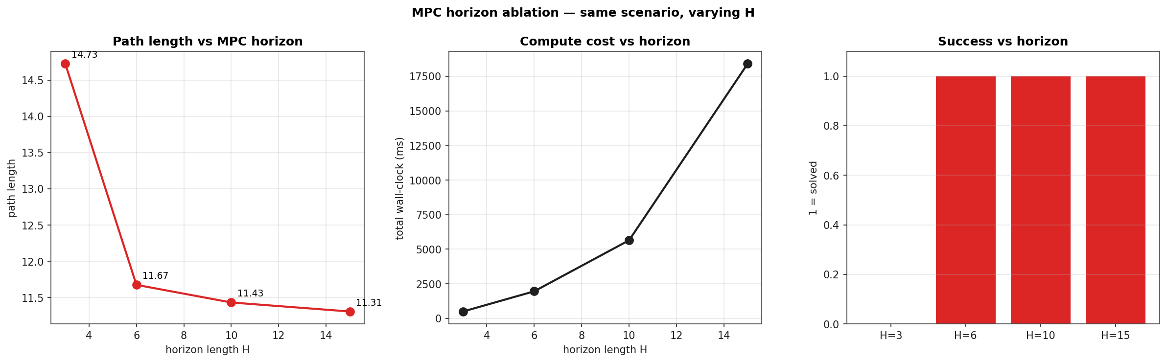
Three-panel ablation: path length vs horizon length, total wall-clock vs horizon, and success indicator vs horizon

The path length saturates near the geometric optimum (≈ 11.31 ≈ 4·√2·2 m for an unobstructed diagonal). H=15 reaches that floor but pays a 17 s total compute bill across the 85-step rollout. In a real-time loop this is the trade-off being engineered: shorter H for higher control rate, longer H for tighter trajectory.

Where MPC sits in the avoidance stack

Reactive PF is the kHz-rate cheap-and-cheerful baseline; it has no foresight and is bitten by local minima.
MPC is the predictive layer: solve a small QP-like problem at the control rate, get coordinated braking and lateral corrections, pay the compute bill.
Multi-agent formation stacks MPC-style logic across agents, each penalising its peers.
For systems with safety guarantees rather than soft penalties, the natural step is CBF-augmented control: collision constraints become hard via control-barrier-function safety filters.